Definition

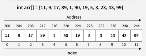
An array is a collection of elements of the same data type, stored at contiguous memory locations. It is one of the most popular and simple data structures used in programming.

• Array Index: Elements in an array are identified by their indexes, which start at 0.
• Array Element: Items stored in an array, accessed using their index.
• Array Length: The length of an array is the number of elements it can contain.

Since all elements in an array are stored in contiguous memory locations, initializing an array allocates memory sequentially. This allows for efficient access and manipulation of elements.

Declaration of Array

Arrays can be declared in different ways depending on the programming language. Below are examples of array declarations in C++:

// Array to store integer elements
int arr[5];      
 
// Array to store character elements
char arr[10];   
 
// Array to store float elements
float arr[20];  

Initialization of Array

Arrays can be initialized in various ways:

int arr[] = { 1, 2, 3, 4, 5 };
char arr[5] = { 'a', 'b', 'c', 'd', 'e' };
float arr[10] = { 1.4, 2.0, 24, 5.0, 0.0 };

Types of Arrays

Arrays can be classified based on two factors:

• Size
• Dimensions

Types of Arrays Based on Size

1. Fixed Size Arrays

   The size of a fixed-size array cannot be altered. The memory for a fixed-size array is allocated at compile-time, and the array size is fixed. If the array is declared with a size that does not match the number of elements, it could lead to wasted memory or insufficient storage.

   // Fixed-size array declared at compile time
   int arr[5]; 
    
   // Fixed-size array declared and initialized
   int arr2[5] = {1, 2, 3, 4, 5}; 

2. Dynamic Size Arrays

   The size of a dynamic array can change during execution, allowing users to add or remove elements as needed. Memory for dynamic arrays is allocated and de-allocated at runtime.

   #include <vector>
    
   // Dynamic Integer Array
   vector<int> v;

Types of Arrays Based on Dimensions

1. One-Dimensional Array (1D Array)

   A one-dimensional array can be imagined as a linear sequence where elements are stored one after another.

   

2. Multi-Dimensional Array

   A multi-dimensional array is an array with more than one dimension. It can be used to store complex data, such as tables. Examples include 2D arrays, 3D arrays, and higher dimensions.

   • Two-Dimensional Array (2D Array or Matrix): A 2D array can be thought of as an array of arrays or a matrix consisting of rows and columns.

     

   • Three-Dimensional Array (3D Array): A 3D array contains three dimensions, and can be considered as an array of 2D arrays.

     

1D Arrays

A one-dimensional array can be viewed as a linear sequence of elements. The size can only be increased or decreased in a single direction.

In a 1D array, only a single row exists, and each element is accessible via its index. In C, array indexing starts from 0, i.e., the first element is at index 0, the second at index 1, and so on, up to n-1 for an array of size n.

Syntax

Declaration of 1D Array

In the declaration, we specify the array's name and size:

elements_type array_name[array_size];

This step reserves memory for the array, but the elements are not initialized and may contain random values. To give the array elements initial values, we need to initialize the array.

Initialization of 1D Array

To assign values to the array, the following syntax is used:

elements_type array_name[array_size] = {value1, value2, ...};

The values are assigned sequentially. For example, the first element will hold value1, the second will hold value2, and so on.

Accessing and Updating Elements of 1D Array

To access an array element, use its index along with the array name:

array_name[index];  // Accessing an element

To update an element, use the assignment operator:

array_name[index] = new_value;  // Updating an element

Note: Make sure the index is within bounds, or else it may result in a segmentation fault.

To access all elements of the array, you can use loops.

Example of One-Dimensional Array

// C++ program to illustrate how to create an array,
// initialize it, update and access elements
#include <iostream>
using namespace std;
 
int main() {
  // Declaring and initializing array (fixed size)
  int arr[5] = {1, 2, 3, 4, 5};
 
  // Printing the array
  for (int i = 0; i < 5; i++) {
    cout << arr[i] << " ";
  }
  cout << endl;
 
  // Updating an element
  arr[3] = 9;
 
  // Printing the updated array
  for (int i = 0; i < 5; i++) {
    cout << arr[i] << " ";
  }
  cout << endl;
 
  return 0;
}

Output:

1 2 3 4 5 
1 2 3 9 5 

Array of Characters (Strings)

A popular use of 1D arrays is for storing textual data, represented as strings. A string is essentially an array of characters terminated by a null character ('\0').

Syntax

char name[] = "This is an example string";

The size of the array is automatically deduced from the assigned string.

Example

// C++ Program to illustrate the use of string
#include <iostream>
#include <string> // Include the string library
 
using namespace std;
 
int main() {
  // Defining a C++ string object
  string str = "This is HPTU Exam Helper";
 
  cout << str << endl; // Use cout for output
 
  return 0;
}

Output:

This is HPTU Exam Helper

2D Arrays

A two-dimensional array (2D array) is a simple form of a multidimensional array. It can be visualized as a set of one-dimensional arrays stacked vertically, forming a table with 'm' rows and 'n' columns. In C, arrays are 0-indexed, meaning that row indices range from 0 to (m-1), and column indices range from 0 to (n-1).

A 2D array with 'm' rows and 'n' columns is created using the following syntax:

type arr_name[m][n];

Where:

• type: The data type of the elements in the array.
• arr_name: The name of the array.
• m: The number of rows.
• n: The number of columns.

For example, to declare a two-dimensional integer array named 'arr' with 10 rows and 20 columns, use:

int arr[10][20];

Initialization of 2D Arrays

A 2D array can be initialized by providing a list of values enclosed in curly braces {}, with values separated by commas. The elements are filled from left to right and top to bottom.

For example:

int arr[3][4] = {0, 1, 2, 3, 4, 5, 6, 7, 8, 9, 10, 11};

Alternatively, you can initialize it as:

int arr[3][4] = {{0, 1, 2, 3}, {4, 5, 6, 7}, {8, 9, 10, 11}};

In this second form, each set of inner braces represents a row. The array will be filled row by row, with each row containing 4 elements.

You can omit the size of the rows in the initializer list. The compiler will deduce it automatically. However, the number of columns must still be specified:

type arr_name[][n] = {…values…};

Note: The number of elements in the initializer list must not exceed the total number of elements in the array.

2D Array Traversal

Traversal refers to accessing each element of the array one by one. To access an element in a 2D array, use row and column indices inside the array subscript operator []:

arr_name[i][j];

Where i is the row index and j is the column index.

To traverse the entire array, use two nested loops: one loop for iterating through rows, and a second nested loop for iterating through columns within each row.

Example of 2D Array Traversal:

#include <iostream>
using namespace std;
 
int main() {
    // Create and initialize a 2D array with 3 rows and 2 columns
    int arr[3][2] = { {0, 1}, {2, 3}, {4, 5} };
 
    // Get the number of rows and columns.  These are fixed at compile time for this style of array.
    const int numRows = 3;
    const int numCols = 2;
 
    // Print each array element's value
    for (int i = 0; i < numRows; ++i) {
        for (int j = 0; j < numCols; ++j) {
            cout << "arr[" << i << "][" << j << "]: " << arr[i][j] << "  ";
        }
        cout << endl;
    }
 
    return 0;
}

Output:

arr[0][0]: 0    arr[0][1]: 1    
arr[1][0]: 2    arr[1][1]: 3    
arr[2][0]: 4    arr[2][1]: 5    

Time Complexity: O(n * m), where 'n' is the number of rows and 'm' is the number of columns.
Auxiliary Space: O(1)

3D Arrays

A three-dimensional (3D) array is a collection of two-dimensional arrays, which can be visualized as multiple 2D arrays stacked on top of each other.

Declaration of 3D Array

A 3D array with 'x' 2D arrays, each having 'm' rows and 'n' columns, can be declared as:

type arr_name[x][m][n];

Where:

• type: The data type of the elements in the array.
• arr_name: The name of the array.
• x: The number of 2D arrays (also called the depth).
• m: The number of rows in each 2D array.
• n: The number of columns in each 2D array.

For example:

int arr[2][2][2];

Initialization of 3D Arrays

Initialization of a 3D array is similar to that of 2D arrays. The key difference is that the number of nested braces increases with the number of dimensions.

Example:

int arr[2][3][2] = {0, 1, 2, 3, 4, 5, 6, 7 , 8, 9, 10, 11};

Alternatively, you can explicitly specify the dimensions using nested braces:

int arr[2][3][2] = { { { 1, 1 }, { 2, 3 }, { 4, 5 } },
                     { { 6, 7 }, { 8, 9 }, { 10, 11 } } };

As with 2D arrays, you can omit the size of the first dimension in the initializer list, and the compiler will deduce it. However, the other dimensions must still be specified.

3D Array Traversal

To access elements in a 3D array, use three indices: one for the depth, one for the row, and one for the column.

arr_name[d][i][j];

Where d is the depth index (representing a specific 2D array), i is the row index within that 2D array, and j is the column index within the 2D array.

To traverse the entire 3D array, use three nested loops: one for the depth (the set of 2D arrays), one for the rows of each 2D array, and one for the columns of each row.

Example of 3D Array Traversal:

#include <iostream>
 
using namespace std;
 
int main() {
    // Create and initialize the 3D array
    int arr[2][3][2] = { { { 1, 1 }, { 2, 3 }, { 4, 5 } },
                           { { 6, 7 }, { 8, 9 }, { 10, 11 } } };
 
    // Get the dimensions of the array.  These are fixed at compile time.
    const int depth = 2;
    const int rows = 3;
    const int cols = 2;
 
    // Loop through the depth
    for (int i = 0; i < depth; ++i) {
        // Loop through the rows of each depth
        for (int j = 0; j < rows; ++j) {
            // Loop through the columns of each row
            for (int k = 0; k < cols; ++k) {
                cout << "arr[" << i << "][" << j << "][" << k << "] = " << arr[i][j][k] << "  ";
            }
            cout << endl;
        }
        cout << endl << endl;
    }
    return 0;
}

Output:

arr[0][0][0] = 1   arr[0][0][1] = 1   
arr[0][1][0] = 2   arr[0][1][1] = 3   
arr[0][2][0] = 4   arr[0][2][1] = 5   

arr[1][0][0] = 6   arr[1][0][1] = 7   
arr[1][1][0] = 8   arr[1][1][1] = 9   
arr[1][2][0] = 10   arr[1][2][1] = 11   

Operations on Arrays

Array Traversal

Array traversal refers to the process of accessing and processing each element of an array sequentially. This is one of the most fundamental operations in programming, as arrays are commonly used data structures for storing multiple elements in a single variable.

When an array is created, it occupies a contiguous block of memory, where elements are stored in an indexed manner. Each element can be accessed using its index, which typically starts from 0 in most programming languages.

For example, consider an array containing five integers:

arr = [10, 20, 30, 40, 50]

Here:

• The first element (10) is at index 0.
• The second element (20) is at index 1.
• The last element (50) is at index 4.

Array traversal means accessing each element from start to end (or sometimes in reverse order), usually using a loop.

Types of Array Traversal

Array traversal can be done in multiple ways depending on the requirement:

• Sequential (Linear) Traversal

  • The most common way of traversing an array.
  • It involves iterating through the array one element at a time from the first index to the last.
  • Used for printing elements, searching, or performing calculations (such as sum or average).

• Reverse Traversal

  • Instead of starting from index 0, the traversal begins from the last element and moves toward the first.
  • Useful when processing elements from the end is needed.

Insertion in Array

Insertion in an array refers to adding a new element at a specific position while maintaining the order of the existing elements. Since arrays have a fixed size in static implementations, inserting an element often requires shifting existing elements to create space.

Arrays are stored in contiguous memory locations, meaning elements are arranged in a sequential block. When inserting a new element, the following steps occur:

1. Identify the Position: Determine where the new element should be inserted.
2. Shift Elements: Move existing elements one position forward to create space for the new element.
3. Insert the New Element: Place the new value in the correct position.
4. Update the Size (if applicable): In dynamic arrays, the size is increased.

For example, consider the array:

arr = [10, 20, 30, 40, 50]

If we want to insert 25 at index 2, the new array will be:

arr = [10, 20, 25, 30, 40, 50]

Here, elements 30, 40, and 50 have shifted to the right to make space.

Types of Insertion

1. Insertion at the Beginning (Index 0)

   • Every element must shift one position to the right.
   • This is the least efficient case for large arrays as it affects all elements.

2. Insertion at a Specific Index

   • Elements after the index shift to the right.
   • If the index is in the middle, half of the array moves.

3. Insertion at the End

   • The simplest case since no shifting is required.
   • Common in dynamic arrays, where the size increases automatically (e.g., Python lists, Java ArrayList).

Deletion in Array

Deletion in an array refers to removing an element from a specific position while maintaining the order of the remaining elements. Unlike linked lists, where deletion is efficient, removing an element from an array requires shifting elements to fill the gap.

Since arrays have contiguous memory allocation, deleting an element does not reduce the allocated memory size. Instead, it involves:

1. Identify the Position: Find the index of the element to be deleted.
2. Shift Elements: Move elements after the deleted element one position to the left.
3. Update the Size (if applicable): In dynamic arrays, the size may be reduced.

For example, consider the array:

arr = [10, 20, 30, 40, 50]

If we delete the element 30 (index 2), the new array will be:

arr = [10, 20, 40, 50]

Here, elements 40 and 50 have shifted left to fill the gap.

Types of Deletion

1. Deletion at the Beginning (Index 0)

   • Every element shifts left by one position.
   • This is the most expensive case as it affects all elements.

2. Deletion at a Specific Index

   • Only elements after the index shift left.
   • If the index is in the middle, half of the array moves.

3. Deletion at the End

   • The simplest case since no shifting is required.
   • The size of the array is reduced (in dynamic arrays).

Searching in Array

Searching in an array refers to finding a specific element in a given list of elements. The goal is to determine whether the element exists in the array and, if so, find its index (position).

Searching is a fundamental operation in programming, used in data retrieval, filtering, and processing.

Types of Searching in an Array

There are two main types of searching techniques in an array:

1. Linear Search (Sequential Search)
   • This is the simplest search algorithm.
   • It traverses the array one element at a time and compares each element with the target value.
   • If a match is found, it returns the index of the element.
   • If the element is not found, the search continues until the end of the array.

Example: Consider an array:

arr = [10, 20, 30, 40, 50]

If we search for 30, the algorithm will:

• Compare 10 with 30 → No match.
• Compare 20 with 30 → No match.
• Compare 30 with 30 → Match found at index 2.

2. Binary Search (Efficient Search for Sorted Arrays)
   • Works only on sorted arrays (in increasing or decreasing order).
   • Uses a divide-and-conquer approach.
   • It repeatedly divides the search space in half until the target element is found.

Working:

1. Find the middle element of the array.
2. If the target is equal to the middle element, return its index.
3. If the target is less than the middle element, search the left half.
4. If the target is greater than the middle element, search the right half.
5. Repeat until the element is found or the search space is empty.

Example: Consider a sorted array:

arr = [10, 20, 30, 40, 50]

If we search for 30:

• Middle element = 30 → Match found!
• The search ends in just one step, making it much faster than linear search.

Sparse Matrices

A matrix is a two-dimensional data structure consisting of $m$ rows and $n$ columns, having a total of $m \times n$ values. If most of the elements in the matrix are zero, it is called a sparse matrix.

• Storage: A sparse matrix contains fewer non-zero elements than zero elements, which means less memory is required to store only the non-zero elements.
• Computing Time: The computational time can be reduced by designing a data structure that only traverses the non-zero elements.

Example

0 0 3 0 4
0 0 5 7 0
0 0 0 0 0
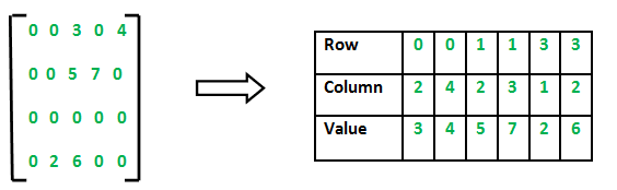
0 2 6 0 0

Representing a sparse matrix using a 2D array results in significant memory wastage, as the zeroes are largely irrelevant. Instead of storing zeroes along with non-zero elements, we only store the non-zero elements. This can be achieved by storing each non-zero element with its corresponding row, column, and value as a triple: (Row, Column, Value).

Sparse matrices can be represented in various ways. The following are two common representations:

1. Array Representation
2. Linked List Representation

Method 1: Using Arrays

A 2D array is used to represent a sparse matrix, with three rows:

• Row: The row index where a non-zero element is located.
• Column: The column index where a non-zero element is located.
• Value: The value of the non-zero element at the specified (row, column) index.

Implementation:

// C++ program for Sparse Matrix Representation using Array
#include <iostream>
using namespace std;
 
int main()
{
    // Assume a 4x5 sparse matrix
    int sparseMatrix[4][5] =
    {
        {0, 0, 3, 0, 4},
        {0, 0, 5, 7, 0},
        {0, 0, 0, 0, 0},
        {0, 2, 6, 0, 0}
    };
 
    int size = 0;
    for (int i = 0; i < 4; i++)
        for (int j = 0; j < 5; j++)
            if (sparseMatrix[i][j] != 0)
                size++;
 
    int compactMatrix[3][size];
 
    // Populating the compact matrix
    int k = 0;
    for (int i = 0; i < 4; i++)
        for (int j = 0; j < 5; j++)
            if (sparseMatrix[i][j] != 0)
            {
                compactMatrix[0][k] = i;
                compactMatrix[1][k] = j;
                compactMatrix[2][k] = sparseMatrix[i][j];
                k++;
            }
 
    for (int i = 0; i < 3; i++)
    {
        for (int j = 0; j < size; j++)
            cout << " " << compactMatrix[i][j];
        cout << "\n";
    }
    return 0;
}

Output:

0 0 1 1 3 3
2 4 2 3 1 2
3 4 5 7 2 6

• Time Complexity: $O(N \times M)$, where $N$ is the number of rows and $M$ is the number of columns in the sparse matrix.
• Auxiliary Space: $O(N \times M)$, where $N$ is the number of rows and $M$ is the number of columns in the sparse matrix.

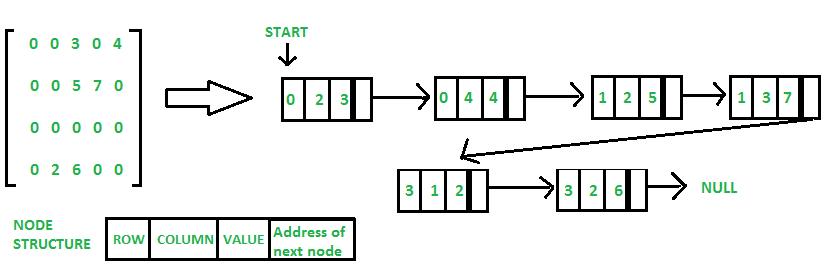
Method 2: Using Linked Lists

In this approach, each node in the linked list contains four fields:

• Row: The row index of the non-zero element.
• Column: The column index of the non-zero element.
• Value: The value of the non-zero element.
• Next Node: A pointer to the next node in the list.

Implementation:

// C++ program for Sparse Matrix Representation using Linked List
#include<iostream>
using namespace std;
 
// Node class to represent a linked list
class Node
{
    public:
    int row;
    int col;
    int data;
    Node *next;
};
 
// Function to create a new node
void create_new_node(Node **p, int row_index, int col_index, int x)
{
    Node *temp = *p;
    Node *r;
 
    // If the linked list is empty, create the first node
    if (temp == NULL)
    {
        temp = new Node();
        temp->row = row_index;
        temp->col = col_index;
        temp->data = x;
        temp->next = NULL;
        *p = temp;
    }
    // If the linked list is already created, append the new node
    else
    {
        while (temp->next != NULL)
            temp = temp->next;
 
        r = new Node();
        r->row = row_index;
        r->col = col_index;
        r->data = x;
        r->next = NULL;
        temp->next = r;
    }
}
 
// Function to print the contents of the linked list
void printList(Node *start)
{
    Node *ptr = start;
    cout << "row_position: ";
    while (ptr != NULL)
    {
        cout << ptr->row << " ";
        ptr = ptr->next;
    }
    cout << endl;
 
    cout << "column_position: ";
    ptr = start;
    while (ptr != NULL)
    {
        cout << ptr->col << " ";
        ptr = ptr->next;
    }
    cout << endl;
 
    cout << "Value: ";
    ptr = start;
    while (ptr != NULL)
    {
        cout << ptr->data << " ";
        ptr = ptr->next;
    }
}
 
// Driver code
int main()
{
    // 4x5 sparse matrix
    int sparseMatrix[4][5] = {{0, 0, 3, 0, 4},
                               {0, 0, 5, 7, 0},
                               {0, 0, 0, 0, 0},
                               {0, 2, 6, 0, 0}};
 
    // Creating the first node of the list (initially NULL)
    Node *first = NULL;
    for (int i = 0; i < 4; i++)
    {
        for (int j = 0; j < 5; j++)
        {
            // Pass only non-zero values
            if (sparseMatrix[i][j] != 0)
                create_new_node(&first, i, j, sparseMatrix[i][j]);
        }
    }
    printList(first);
 
    return 0;
}

Output:

row_position: 0 0 1 1 3 3
column_position: 2 4 2 3 1 2
Value: 3 4 5 7 2 6

• Time Complexity: $O(N \times M)$, where $N$ is the number of rows and $M$ is the number of columns in the sparse matrix.
• Auxiliary Space: $O(K)$, where $K$ is the number of non-zero elements.

Other Representations

• Dictionary Representation: The row and column numbers are used as keys, and the matrix entries are the values. This method saves space but is inefficient for sequential access of elements.
• List of Lists: The idea is to create a list for each row, where each item in the list corresponds to a non-zero element. These lists can be sorted by column numbers to optimize access.

Structures and Arrays of Structures

In programming, a structure is a composite data type that groups multiple variables of potentially different data types into a single unit. An array of structures is a collection of such structures stored sequentially.

Structures

• Definition: A structure is a user-defined data type that groups variables of different data types together.
• Purpose: Structures are used to represent complex data entities, such as a student record with roll number, name, and grades.
• Example:

struct Student {
    int roll_number;
    char name[50];
    float marks;
};

• Memory Allocation: Structures do not require consecutive memory locations.

Arrays

• Definition: An array is a collection of elements of the same data type, stored in contiguous memory locations.
• Purpose: Arrays are used to manage collections of data, such as lists of integers or strings.
• Example:

int numbers[5];  // An array to store 5 integers

• Memory Allocation: Arrays store data in contiguous memory locations, meaning the memory blocks are assigned consecutively.

Arrays of Structures

• Definition: An array of structures combines arrays and structures, allowing you to store a collection of records, where each record is a structure containing multiple data fields.
• Example:

struct Student {
    int roll_number;
    char name[50];
    float marks;
};
struct Student students[10];  // An array to store 10 student records

• How it works: You define a structure (like Student), then create an array of that structure type (like students[10]). Each array element is a structure representing a single record.

Here is an example code for array of structures.

Key Differences

• Data Type: Structures can contain variables of different data types, whereas arrays can only store elements of the same data type.
• Memory Allocation: Structures do not require contiguous memory, while arrays store data contiguously.
• Accessibility: To access members of a structure, use the dot operator (e.g., student.name), whereas array elements are accessed by their index (e.g., numbers[0]).