Definition
The term algorithm refers to a finite set of well-defined rules or instructions to be followed in calculations or other problem-solving operations. It can also be defined as a procedure for solving a mathematical problem in a finite number of steps, often involving recursion.
In essence, an algorithm is a sequence of finite steps designed to solve a specific problem.
Use of Algorithms
Algorithms are fundamental to various disciplines and have a wide range of applications. Some key areas include:
- Computer Science: Algorithms are the foundation of programming, used in everything from basic sorting and searching to advanced tasks like artificial intelligence and machine learning.
- Mathematics: Algorithms solve problems such as finding the shortest path in a graph or optimizing a system of equations.
- Operations Research: Algorithms aid in optimization and decision-making in areas like logistics, transportation, and resource management.
- Artificial Intelligence: Algorithms power intelligent systems capable of image recognition, natural language processing, and decision-making.
- Data Science: Algorithms help analyze, process, and derive insights from large datasets in fields like healthcare, finance, and marketing.
As technology evolves, algorithms continue to play an increasingly important role across new and emerging fields.
From a data structure perspective, important categories of algorithms include:
- Search – To locate an item within a data structure.
- Sort – To arrange items in a specific order.
- Insert – To add an item to a data structure.
- Update – To modify an existing item in a data structure.
- Delete – To remove an item from a data structure.
Characteristics
Just as one follows a standard recipe for cooking instead of arbitrary instructions, not every set of written steps qualifies as an algorithm. To be considered an algorithm, a set of instructions must meet the following characteristics:
- Clear and Unambiguous: Every step should be precise and lead to a single, definite interpretation.
- Well-Defined Inputs: Inputs, if required, should be clearly specified. An algorithm may take zero or more inputs.
- Well-Defined Outputs: At least one output must be produced, and it should be clearly defined.
- Finite-ness: The algorithm must terminate after a finite number of steps.
- Feasible: The steps must be practical and executable using available resources. The algorithm should not rely on future or imaginary technologies.
- Language Independent: The algorithm should consist of generic steps, independent of any specific programming language. It should yield consistent results regardless of the implementation language.
Properties of an Algorithm:
- It terminates after a finite time.
- It produces at least one output.
- It accepts zero or more inputs.
- It is deterministic, yielding the same output for the same input.
- Each step is effective, meaning it performs a meaningful task.
Advantages of Algorithms
- Easy to understand and follow.
- Presents a step-by-step solution to a problem.
- Breaks the problem into manageable parts, aiding in easier implementation.
Disadvantages of Algorithms
- Time-consuming to write, especially for complex problems.
- Can be difficult to express complex logic.
- Representation of control structures like loops and branching can be challenging.
Development of an Algorithm
Developing an algorithm in the context of data structures involves creating a systematic procedure to solve a computational problem, often involving data stored in structured formats like arrays, linked lists, or trees.
-
Problem Understanding
- Define the Problem: Clearly identify the task to be solved.
- Identify Constraints: Consider limitations on data size, time, or resources.
- Determine Inputs and Outputs: Understand what data the algorithm will receive and what results are expected.
-
Algorithm Design
- Select Data Structures: Choose suitable structures (arrays, trees, graphs, etc.) to handle the data effectively.
- Design the Procedure: Develop a logical, step-by-step process to solve the problem using the selected data structure.
- Explore Algorithm Paradigms: Consider approaches like divide-and-conquer, greedy methods, or dynamic programming.
- Analyze Complexity: Evaluate time and space requirements (e.g., O(n), O(log n)).
-
Implementation and Testing
- Translate into Code: Implement the algorithm using a programming language and appropriate data structures.
- Perform Testing: Run the program with various inputs to ensure reliability and correctness.
- Debug and Optimize: Fix issues and improve efficiency.
-
Documentation
- Document the Algorithm: Clearly explain how it works, its inputs and outputs, and any limitations.
- Document the Code: Provide code-level explanations for better maintainability.
Analysis of Complexity
Complexity analysis is a method used to evaluate the performance of an algorithm, particularly the time and space it requires relative to the size of its input. This analysis is independent of the underlying machine, programming language, or compiler.
- It helps determine the time and memory resources needed for execution.
- It enables comparison between different algorithms across varying input sizes.
- It offers insight into the computational difficulty of a problem.
- Complexity is often described in terms of time (execution speed) and space (memory usage).
Time Complexity
To compare different algorithms, it's more effective to use time complexity rather than actual runtime, which can vary based on hardware or implementation details.
Time complexity describes the number of operations an algorithm performs relative to input size. Since each operation consumes some amount of time, the total number of operations serves as an abstract representation of time.
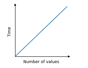
For example, if the time taken increases proportionally with the size of the input, the relationship is linear and can be visualized as such on a graph:
To compute time complexity, it's assumed that each operation takes a constant time c. The total time is then derived from the number of operations for input size N.
Example: Suppose we need to check if a pair (X, Y) exists in an array A of N elements such that their sum is equal to Z. A straightforward approach is to check all possible pairs:
#include <iostream>
using namespace std;

bool findPair(int a[], int n, int z)
{
    for (int i = 0; i < n; i++)
        for (int j = 0; j < n; j++)
            if (i != j && a[i] + a[j] == z)
                return true;
    return false;
}

int main()
{
    int a[] = { 2, -12, 13, 7, 0 };
    int z = 0;
    int n = sizeof(a) / sizeof(a[0]);

    if (findPair(a, n, z))
        cout << "True";
    else
        cout << "False";
    return 0;
}
Output
FalseSpace Complexity
Solving problems using a computer requires memory to store intermediate data and final results during execution. Space complexity refers to the amount of memory an algorithm needs relative to the size of the input.
Space complexity measures how much additional memory is required to execute an algorithm, and is typically expressed as a function of input length.
Example: To find the frequency of each element in an array, memory is needed to store the frequency count:
- If an array of size
nis created, it requiresO(n)space. - A two-dimensional array of size
n × nneedsO(n²)space.
To estimate memory usage, we consider two components:
- Fixed Part: Independent of input size. This includes memory for constants, variables, and instructions.
- Variable Part: Depends on the input size. This includes dynamic memory used for data structures like stacks, arrays, or recursion.
For instance, adding two scalar numbers requires only one additional memory location, so the space complexity is constant: S(n) = O(1).
#include <bits/stdc++.h>
using namespace std;

void countFreq(int arr[], int n)
{
    unordered_map<int, int> freq;

    for (int i = 0; i < n; i++)
        freq[arr[i]]++;

    for (auto x : freq)
        cout << x.first << " " << x.second << endl;
}

int main()
{
    int arr[] = { 1, 2, 2, 1, 1, 2, 3, 2 };
    int n = sizeof(arr) / sizeof(arr[0]);

    countFreq(arr, n);
    return 0;
}
Output
3 1
2 4
1 3
Order of Growth
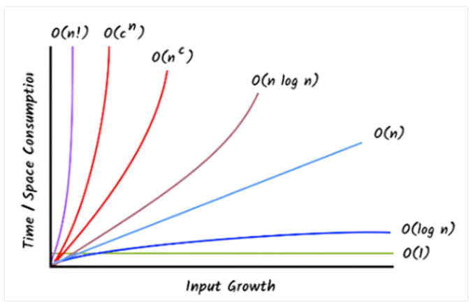
Order of growth explains how an algorithm’s runtime or memory usage increases as the size of the input grows. Instead of focusing on the actual time, it looks at how fast the resource requirements grow. This helps compare algorithms, especially with large inputs.
Some common types of growth:
- O(1) - Constant time: stays the same no matter the input.
- O(log n) - Logarithmic time: grows slowly as input grows.
- O(n) - Linear time: grows in direct proportion to input.
- O(n²) - Quadratic time: grows rapidly as input doubles.
- O(2ⁿ) - Exponential time: grows very fast, not scalable.
Key Concepts:
- Asymptotic Analysis: Focuses on what happens as input size becomes very large (approaches infinity).
- Big O Notation: Describes the worst-case growth.
- Why It Matters: Helps choose efficient algorithms for large data.
- Other Notations:
- Big Ω (Omega) shows the best case.
- Big Θ (Theta) shows the average/tight bound.
Here’s a table showing common time complexities:
| Order | Big-Theta | Example |
|---|---|---|
| Constant | Indexing an item in a list | |
| Logarithmic | Repeatedly halving a number | |
| Linear | Summing a list | |
| Quadratic | Summing each pair of numbers in a list | |
| Exponential | Visiting each node in a binary tree |
Asymptotic Notation
Asymptotic notation is a set of mathematical tools used in computer science to describe the efficiency and scalability of algorithms. It provides a high-level understanding of an algorithm’s behavior, particularly as the input size increases.
In simple terms, it helps determine an algorithm’s performance in the best-case (minimum time), average-case, and worst-case (maximum time) scenarios by analyzing the running time of each operation using mathematical expressions.
Example:
Problem Statement:
If the time taken by two programs is T(n) = a·n + b and V(n) = c·n² + d·n + e, which program is more efficient?
Solution:
The linear algorithm T(n) is always asymptotically more efficient than the quadratic algorithm V(n). For any positive constants a, b, c, d, and e, there exists a value of n such that:
c·n² + d·n + e ≥ a·n + bHence, V(n) will eventually take more time than T(n) as n grows.
Note:
- Rule of Thumb: The slower the asymptotic growth rate, the better the algorithm.
- Input-Bound Analysis: Asymptotic analysis focuses solely on input size; all other factors are considered constant.
- Focus on Growth: It analyzes the growth of f(n) as n → ∞, so small values of n are often ignored.
- Purpose: The goal is not to compute the exact runtime but to understand how the function behaves as the input grows large.
Importance of Asymptotic Notation
- Categorizes algorithms by their performance as input size grows.
- Helps assess how algorithms scale with increasing data complexity.
- Predicts behavior under various conditions, assisting in performance forecasting.
- Enables fair comparison of different algorithms by abstracting away hardware and implementation details.
- Aids in making informed decisions about algorithm selection based on efficiency and resource limitations.
Types of Asymptotic Notation
- Big O Notation (O) – Describes the upper bound (worst-case scenario).
- Omega Notation (Ω) – Describes the lower bound (best-case scenario).
- Theta Notation (Θ) – Describes the tight bound (average-case or exact growth).
Big O Notation
A function f(n) is said to be O(g(n)) if there exist positive constants and such that for all . This means that for sufficiently large values of n, the function f(n) does not grow faster than g(n) up to a constant factor. Big O notation describes the upper bound of an algorithm’s time or space complexity. It captures the worst-case performance as input size increases.
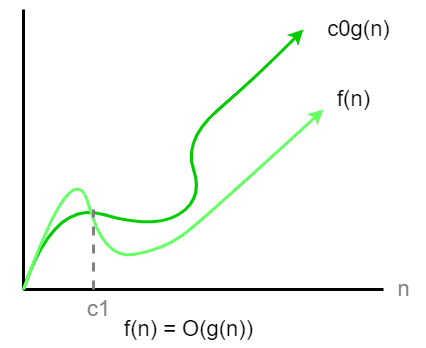
Mathematical Definition:
O(g(n)) = {f(n): ∃ positive constants c₀ and c₁ such that 0 ≤ f(n) ≤ c₀·g(n) for all n ≥ c₁}Example:
f(n) = n² + n + 1
g(n) = n²
We can find a constant c such that:
n² + n + 1 ≤ c·n²Thus, the time complexity is O(n²), since n² dominates the growth.
Omega Notation
A function f(n) is said to be Ω(g(n)) if there exist positive constants and such that
for all .
This means that for sufficiently large values of n, the function f(n) grows at least as fast as g(n) up to a constant factor.
Omega notation describes the lower bound of an algorithm’s time or space complexity. It captures the best-case performance as the input size increases.
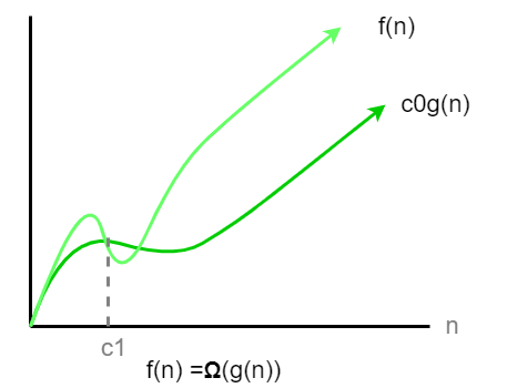
Mathematical Definition:
Ω(g(n)) = {f(n): ∃ positive constants c₀ and c₁ such that 0 ≤ c₀·g(n) ≤ f(n) for all n ≥ c₁}Examples:
f(n) = n² + n → Ω(n²)
f(n) = 100n + log(n) → Ω(n)
Theta Notation
A function f(n) is said to be Θ(g(n)) if there exist positive constants , , and such that
for all .
This means that for sufficiently large values of n, the function f(n) grows at the same rate as g(n) up to constant factors.
Theta notation describes the tight bound of an algorithm’s time or space complexity. It provides an accurate representation of the algorithm’s growth rate by bounding it from both above and below.
.
Theta notation provides a tight bound, meaning it bounds a function from both above and below. It represents the exact asymptotic behavior.
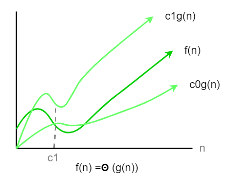
Mathematical Definition:
Θ(g(n)) = {f(n): ∃ positive constants c₀, c₁, and c₂ such that 0 ≤ c₀·g(n) ≤ f(n) ≤ c₁·g(n) for all n ≥ c₂}Limitations of Asymptotic Analysis
- Depends on Large Input Size: Real-world inputs may not always be large enough to reflect asymptotic behavior.
- Ignores Constant Factors: Only the dominant term matters; smaller terms and constants are discarded.
- No Exact Timing: It shows growth patterns, not precise execution time.
- Doesn’t Consider Memory (Unless Specified): Focuses mainly on time complexity.
- Ignores Coefficients of Dominant Terms: Two functions with the same dominant term are treated equally, regardless of coefficients.
- Not Universally Applicable: Some algorithms (e.g., randomized or with complex control flows) don't suit traditional asymptotic analysis well.
Difference Between Big O, Big Omega, and Big Theta
| S.No. | Big O (O) | Big Omega (Ω) | Big Theta (Θ) |
|---|---|---|---|
| 1. | Describes upper bound (≤) | Describes lower bound (≥) | Describes tight bound (bounded above and below) |
| 2. | Upper limit of growth | Minimum guaranteed growth | Exact growth rate up to constant factors |
| 3. | Worst-case analysis | Best-case analysis | Tight-bound analysis (both best and worst cases match) |
| 4. | Used for maximum time/space | Used for minimum time/space | Applies only when upper and lower bounds are tightly coupled |
| 5. | for all | for all | for all |
Obtaining the Complexity
To determine the complexity of an algorithm, analyze how its execution time or memory usage grows with input size. This is often expressed using Big O notation to understand asymptotic behavior.
1. Time Complexity
Time complexity represents the time an algorithm takes to complete, expressed as a function of input size.
Common Complexities:
- O(1): Constant time – independent of input size.
- O(log n): Logarithmic time – grows slowly with input.
- O(n): Linear time – grows directly with input.
- O(n log n): Often found in efficient sorting algorithms.
- O(n²): Quadratic time – grows proportionally to input squared.
- O(2ⁿ): Exponential time – grows very rapidly with input size.
2. Space Complexity
Space complexity measures the memory used by an algorithm, also in terms of input size.
Examples:
- O(1): Constant memory usage.
- O(n): Linear memory usage.
- O(n²): Memory grows quadratically with input size.
Example: Determining Time Complexity
void iterateArray(int arr[], int size) {
    for (int i = 0; i < size; i++) {
        // Some operation
    }
}- Basic Operation: Iteration through the array.
- Number of Operations: n (length of the array).
- Time Complexity: O(n)