Cauchy's Theorem

Cauchy's Theorem is one of the central results in complex analysis. It provides a foundation for several powerful results in the study of analytic functions, such as Cauchy's Integral Formula, the Residue Theorem, and the Laurent series.

Let $f(z)$ be a function that is analytic (holomorphic) inside and on a simple, closed contour C in a domain D. Then the contour integral of f(z) around C is zero:

$\oint_C f(z) \, dz = 0$

• Analytic (Holomorphic): A function $f(z)$ is said to be analytic at a point $z_0$ if it has a derivative at $z_0$ and in some neighborhood around $z_0$. In other words, $f(z)$ is infinitely differentiable in this region.

• Simply Connected Domain: A domain D is said to be simply connected if any closed contour within D can be continuously deformed to a point without leaving D. This implies that the domain contains no "holes".

• Contour: A contour C is a piecewise smooth, closed curve in the complex plane. Cauchy's Theorem requires that C be simple, meaning it does not intersect itself.

Cauchy's Integral Formula

Cauchy's Integral Formula

Let f(z) be a function that is analytic inside and on a simple closed contour C in a domain D, and let $z_0$ be any point inside C. Then for any $z_0$ inside C, the value of the function $f(z_0)$ is given by the contour integral:

$f(z_0) = \frac{1}{2\pi i} \oint_C \frac{f(z)}{z - z_0} \, dz$

This is Cauchy's Integral Formula.

Key terms

• Analytic (Holomorphic): A function f(z) is analytic at a point if it has a derivative at that point and at all points in some neighborhood of that point.
• Contour C: A simple, closed, and piecewise smooth curve in the complex plane.
• $z_0$: Any point inside the contour C.

The formula can be generalized to give the value of any derivative of $f(z)$ inside the contour C.

Generalized Formula for Derivatives: Let f(z) be analytic inside and on C, and let $z_0$ be a point inside C. The n-th derivative of f(z) at $z_0$ is given by:

$f^{(n)}(z_0) = \frac{n!}{2\pi i} \oint_C \frac{f(z)}{(z - z_0)^{n+1}} \, dz$

This result allows us to calculate higher-order derivatives of an analytic function at points inside C based solely on the values of the function on the contour.

Taylor's and Laurent's Series

Taylor's Series:

If f(z) is analytic inside a circle C with centre at a, then for z inside C,

$f(z) = f(a) + f'(a)(z - a) + \frac{f''(a)}{2!}(z - a)^2 + \dots + \frac{f^{(n)}(a)}{n!}(z - a)^n + \dots \; \; \; \; \text{(i)}$

Proof:

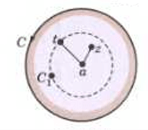
Let z be any point inside C. Draw a circle $C_1$ with centre at a enclosing z (Fig.).

Let t be a point on $C_1$. We have

$\frac{1}{t - z} = \frac{1}{t - a} \left( 1 - \frac{z - a}{t - a} \right)^{-1}$

$= \frac{1}{t - a} \left[ 1 + \frac{z - a}{t - a} + \left( \frac{z - a}{t - a} \right)^2 + \dots + \left( \frac{z - a}{t - a} \right)^n + \dots \right] \; \; \; \; \; \text{(ii)}$

As $|z - a| < |t - a|$, i.e., $\left| \frac{z - a}{t - a} \right| < 1$, this series converges uniformly. So, multiplying both sides of (ii) by f(t), we can integrate over $C_1$.

Thus,

$\oint_C \frac{f(t)}{t - z} dt = \oint_{C_1} \frac{f(t)}{t - a} \left[ 1 + \frac{z - a}{t - a} + \dots + \left( \frac{z - a}{t - a} \right)^n + \dots \right] dt \; \; \; \; \text{(iii)}$

Since $f(t)$ is analytic on and inside $C_1$, therefore, applying the formulae, we get (i) which is known as Taylor's series.

Laurent's Series:

If $f(z)$ is analytic in the ring-shaped region $R$ bounded by two concentric circles $C$ and $C_1$ of radii $r$ and $r_1$ ($r > r_1$) and with centre at $a$, then for all $z$ in $R$

$f(z) = a_0 + a_1(z - a) + a_2(z - a)^2 + \cdots + a_n (z - a)^n + a_{-1}(z - a)^{-1} + a_{-2}(z - a)^{-2} + \cdots$

where

$a_n = \frac{1}{2\pi i} \oint_\Gamma \frac{f(t)}{(t - a)^{n+1}} \, dt,$

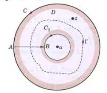
$\Gamma$ being any curve in $R$, encircling $C_1$ (as in Fig.).

Proof: Introduce cross-out $AB$, then $f(z)$ is analytic in the region $D$ bounded by $AB$, $C$, described clockwise, $BA$ and $C_1$ described anti-clockwise (Fig. ). Then if $z$ be any point in $D$, we have

$f(z) = \frac{1}{2\pi i} \left( \oint_C \frac{f(t)}{t - z} \, dt + \int_{B}^{A} \frac{f(t)}{t - z} \, dt + \oint_{C_1} \frac{f(t)}{t - z} \, dt + \int_{A}^{B} \frac{f(t)}{t - z} \, dt \right)$

$= \frac{1}{2\pi i} \oint_C \frac{f(t)}{t - z} \, dt - \oint_{C_1} \frac{f(t)}{t - z} \, dt \; \; \; \; \text{(i)}$

where both $C$ and $C_1$ are described anti-clockwise in (i) and integrals along $AB$ and $BA$ cancel (Fig.).

For the first integral in (i), expanding $1/(t - z)$ , we get

$\oint_C \frac{f(t)}{t - z} \, dt = \sum_{n=1}^{\infty} (z - a)^{n-1} \oint_C \frac{f(t)}{(t - a)^{n+1}} \, dt$

$= \sum_{n=1}^{\infty} a_n (z - a)^n$

where

$a_n = \frac{1}{2\pi i} \oint_C \frac{f(t)}{(t - a)^{n+1}} \, dt$

For the second integral in (i), let $t$ lie on $C_1$. Then we write

$\frac{1}{t - z} = \frac{1}{(t - a) - (z - a)} = \frac{1}{t - a} \left( 1 - \frac{z - a}{t - a} \right)^{-1}$

$= \frac{1}{t - a} \left[ 1 + \frac{z - a}{t - a} + \frac{(z - a)^2}{(t - a)^2} + \cdots + \frac{(z - a)^{n-1}}{(t - a)^{n-1}} + \cdots \right]$

As $|t - a| < |z - a|$, i.e., $|(t - a)/(z - a)| < 1$, this series converges uniformly. So multiplying both sides by $f(t)$ and integrating over $C_1$, we get

$\frac{1}{2\pi i} \oint_{C_1} \frac{f(t)}{t - z} \, dt = \frac{1}{2\pi i} \sum_{n=1}^{\infty} \oint_{C_1} \frac{f(t)}{(t - a)^{n+1}} \, dt \cdot (z - a)^{-n}$

$= \sum_{n=1}^{\infty} a_{-n} (z - a)^{-n}$

where

$a_{-n} = \frac{1}{2\pi i} \oint_{C_1} \frac{f(t)}{(t - a)^{n+1}} \, dt$

Substituting from (ii) and (iii) in (i), we get

$f(z) = \sum_{n=0}^{\infty} a_n (z - a)^n + \sum_{n=1}^{\infty} a_{-n} (z - a)^{-n}$

$= \sum_{n=-\infty}^{\infty} a_n (z - a)^n \; \; \; \; \text{(iv)}$

Now $f(t)(t - a)^{-n-1}$ being analytic in the region between $C$ and $\Gamma$, we can take the integral giving $a_n$ over $\Gamma$. Similarly we can take the integral giving $a_{-n}$ over $\Gamma$. Hence (iv) can be written as

$f(z) = \sum_{n=-\infty}^{\infty} a_n (z - a)^n \quad \text{where} \quad a_n = \frac{1}{2\pi i} \oint_\Gamma \frac{f(t)}{(t - a)^{n+1}} \, dt$

which is known as Laurent's series.

Zeros and Singularities

Zeros

A zero of an analytic function $f(z)$ is that value of $z$ for which $f(z) = 0$. If $f(z)$ is analytic in the neighbourhood of a point $z = a$, then by Taylor's theorem

$f(z) = a_0 + a_1 (z - a) + a_2 (z - a)^2 + \cdots + a_n (z - a)^n + \cdots \quad \text{where} \quad a_n = \frac{f^{(n)}(a)}{n!}$

If $a_0 = a_1 = a_2 = \cdots = a_{m-1} = 0$ but $a_m \neq 0$, then $f(z)$ is said to have a zero of order $m$ at $z = a$. When $m = 1$, the zero is said to be simple. In the neighbourhood of zero $(z = a)$ of order $m$,

$f(z) = a_m (z - a)^m + a_{m+1} (z - a)^{m+1} + \cdots$

$= (z - a)^m \phi(z) \quad \text{where} \quad \phi(z) = a_m + a_{m+1} (z - a) + \cdots$

Then $\phi(z)$ is analytic and non-zero in the neighbourhood of $z = a$.

Singularities

Singularities of an analytic function:

We have already defined a singular point of a function as the point at which the function ceases to be analytic.

(i) Isolated singularity: If $z = a$ is a singularity of $f(z)$ such that $f(z)$ is analytic at each point in its neighbourhood (i.e., there exists a circle with centre at $a$ which has no other singularity), then $z = a$ is called an isolated singularity.

In such a case, $f(z)$ can be expanded in a Laurent’s series around $z = a$, giving

$f(z) = a_0 + a_1 (z - a) + a_2 (z - a)^2 + \cdots + a_n (z - a)^{-1} + a_{-2} (z - a)^{-2} + \cdots \; \; \; \; \text{(1)}$

For example, $f(z) = \cot(\pi z)$ is not analytic where $\tan(\pi z) = 0$, i.e., at the points $\pi z = 4\pi$ or $z = 1/n$ $(n = 1, 2, 3, \dots)$.

Thus $z = 1, 1/2, 1/3, \dots$ are all isolated singularities as there is no other singularity in their neighbourhood.

But when $n$ is large, $z = 0$ is such a singularity that there are an infinite number of other singularities in its neighbourhood. Thus $z = 0$ is the non-isolated singularity of $f(z)$.

(ii) Removable singularity: If all the negative powers of $(z - a)$ in (1) are zero, then

$f(z) = \sum_{n=0}^{\infty} a_n (z - a)^n$

Here the singularity can be removed by defining $f(z)$ at $z = a$ in such a way that it becomes analytic at $z = a$. Such a singularity is called a removable singularity.

Thus if $f(z)$ exists finitely, then $z = a$ is a removable singularity.

(iii) Poles: If all the negative powers of $(z - a)$ in (i) after the $n$th are missing, then the singularity at $z = a$ is called a pole of order $n$.

A pole of first order is called a simple pole.

(iv) Essential singularity: If the number of negative powers of $(z - a)$ in (1) is infinite, then $z = a$ is called an essential singularity. In this case, $\lim_{z \to a} f(z)$ does not exist.

Cauchy's Residue Theorem

Residues

The coefficient of $(z - a)^{-1}$ in the expansion of $f(z)$ around an isolated singularity is called the residue of $f(z)$ at that point. Thus in the Laurent’s series expansion of $f(z)$ around $z = a$, i.e.,

$f(z) = a_0 + a_1 (z - a)^{-1} + a_2 (z - a)^{-2} + \cdots,$

the residue of $f(z)$ at $z = a$ is $a_{-1}$.

$\therefore \quad \operatorname{Res} f(a) = \frac{1}{2\pi i} \oint_C f(z) \, dz$

i.e.,

$\oint_C f(z) \, dz = 2 \pi i \operatorname{Res} f(a). \; \; \; \; \text{(1)}$

Cauchy's Residue Theorem

If $f(z)$ is analytic in a closed curve $C$ except at a finite number of singular points within $C$, then

$\oint_C f(z) \, dz = 2 \pi i \times$ (sum of the residues at the singular points within C).

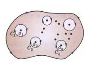
Let us surround each of the singular points $a_1, a_2, \dots, a_n$ by a small circle such that it encloses no other singular point (Fig.). Then these circles $C_1, C_2, \dots, C_n$ together with $C$ form a multiply connected region in which $f(z)$ is analytic.

Applying Cauchy’s theorem, we have

$\oint_C f(z) \, dz = \oint_{C_1} f(z) \, dz + \oint_{C_2} f(z) \, dz + \dots + \oint_{C_n} f(z) \, dz$

$= 2 \pi i \left[ \operatorname{Res} f(a_1) + \operatorname{Res} f(a_2) + \dots + \operatorname{Res} f(a_n) \right]$

which is the desired result.